|
|
R1 - Baseline ocean observations and contemporary modeling
In order to develop the project database (T1.1), data were collated from: the World Ocean Database (WOD Ocean Station Data, [Boyer et al., 2013]), the International Council for the Exploration of the Sea Dataset on Ocean Hydrography (ICES, Copenhagen, 2013), the Global Ocean Data Analysis Project, version 2 (GLODAPv2, [Key et al., 2015; Olsen et al., 2016]), the CARINA Iceland and Irminger Sea Time Series version 2 [Olafsson et al., 2009a, 2009b], and a set of cruise data from the Kara Sea provided by the Shirshov Institute on Oceanology (hereafter the “Russian data”). In order to perform data quality control (T1.2), for GLODAPv2 and CARINA data we required primary QC flag = 0 (‘approximated’), 2 (‘good’), or 6 (‘replicated’) [Key et al., 2010; Olsen et al., 2016], and for the Russian data we excluded any values flagged as extrapolated to depth. We used data from (WOD, ICES, GLODAPv2, Russian) datasets for (T, S) and from (GLODAPv2, CARINA, Russian) datasets for CO2 chemistry variables (D 1.1.).
In order to maximize the CO2 chemistry data coverage, the GLODAPv2 and CARINA datasets were merged and parsed, and equilibrium values were recalculated using CO2SYS.m with constants from [Millero, 2010] and [Uppström, 1974; Dickson, 1990] and missing silicate/phosphate data filled by kernel-smoothing in 3D (x,y,z) [Hastie et al., 2009]. We refer to this extended dataset as GLODAPv2E. The Russian CO2 chemistry data originally included (Alk, pH) pairs with pH reported on the NBS scale. Again, CO2SYS.m with the aforementioned constants was used to convert pH to total scale and to calculate the corresponding (DIC, Ω). To estimate bottom water values we extrapolated profiles to estimated seafloor depths by kernel smoothing. Water depth was estimated by interpolating high-resolution bathymetry products (the 500m-resolution IBCAOv3 [Jakobsson et al., 2012] where available, otherwise the 2-minute ETOPOv2 [National Geophysical Data Center, 2006]) and corrected to the maximum sampled depth wherever this exceeded the interpolated depth. Variables were collated into the final project dataset (D1.1, Figure 1).
The SINMOD biogeochemical model was run for a hindcast period (1979-2008) using reanalysis forcing from ECMWF (T1.5, D1.3) and boundary conditions from the Bergen Climate Model, bias-corrected using the CARINA data (T1.7, D1.5) (see Slagstad et al., 2015 and Bellerby et al., 2012 for details). This output was subsequently used to develop GIS maps (T1.3, D1.2).
In order to transfer the data to the model grid and estimate model bias (T1.4), SINMOD bottom water output was first linearly interpolated in 3D (x,y,t) to the observational data. These matchups allowed us to validate the model (T1.6, Figure 1). For (T,S), horizontal coverage was sufficient to estimate bias by kernel-smoothing the (model minus data) residuals (Figure 2); for CO2 chemistry variables, the bias was modelled as spline functions of the model bathymetry (Figure 3). We then produced bias-corrected estimates of present-day bottom water state (D1.4) by subtracting the bias estimates from the model output.
|
|
|
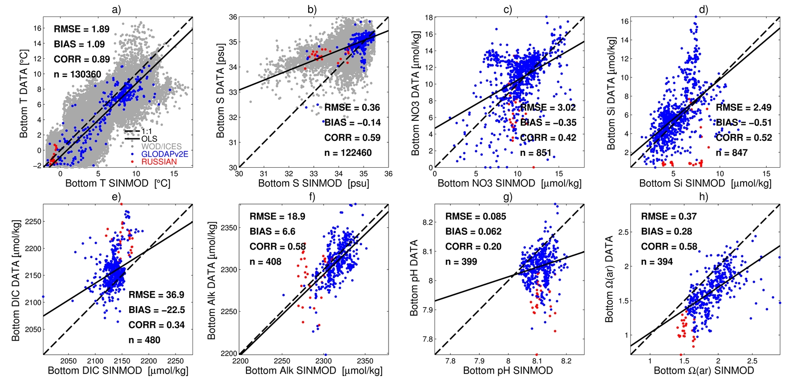
Figure 1. Point-to-point skill assessment for SINMOD bottom water variables. T = temperature (a), S = salinity (b), NO3 = nitrate (c), Si = silicate (d), DIC = dissolved inorganic carbon (e), Alk = total alkalinity (f), pH = total scale pH (g), Ω(ar) = aragonite saturation state (h). Skill was computed as RMSE = root-mean-square error, BIAS = mean(model - data), and CORR = Pearson correlation (n is the number of model-data pairs). Dashed black lines are 1:1 and solid black lines are from ordinary least squares linear regression. Data (points) are from WOD / ICES datasets (grey), the extended GLODAPv2 dataset (blue), and the Russian Kara Sea dataset (red).
|
|
|
|
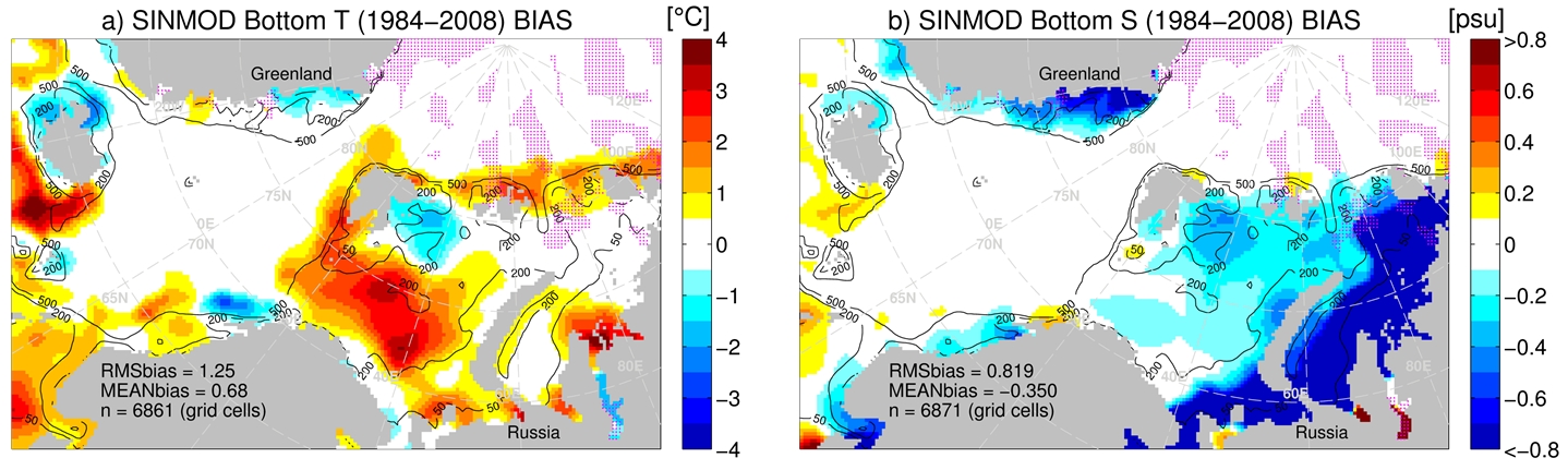
Figure 2. SINMOD regional biases in bottom temperature (a) and bottom salinity (b). Magenta dots mark grid cells for which data coverage was lacking (no data within two bandwidths of the grid cell center). RMSbias and MEANbias show the root-mean-square and mean bias over all unmarked grid cells at model depths 50–500 m and “n” shows the number of such cells. Black lines show 50, 200, and 500 m depth contours.
|
References:
-
Bellerby, R. G. J., A. Silyakova, G. Nondal, D. Slagstad, J. Czerny, T. de Lange, A. Ludwig, and B. Discussions (2012), Marine carbonate system evolution during the EPOCA Arctic pelagic ecosystem experiment in the context of simulated Arctic ocean acidification, Biogeosciences Discuss., 9(11), 15541–15565.
-
Boyer, T. P. et al. (2013), World Ocean Database 2013, Sydney Levitus, Ed.; Alexey Mishonoc, Tech. Ed., NOAA Atlas(72), 209 pp.
-
Dickson, A. G. (1990), Standard potential of the reaction: AgCl(s) + 12H2(g) = Ag(s) + HCl(aq), and and the standard acidity constant of the ion HSO4− in synthetic sea water from 273.15 to 318.15 K, J. Chem. Thermodyn., 22(2), 113–127.
-
Hastie, T., R. Tibshirani, and J. Friedman (2009), The Elements of Statistical Learning: Data Mining, Inference, and Prediction., 2nd ed., Springer-Verlag, New York.
-
Jakobsson, M. et al. (2012), The International Bathymetric Chart of the Arctic Ocean (IBCAO) Version 3.0, Geophys. Res. Lett., 39, L12609.
-
Key, R. M. et al. (2010), The CARINA data synthesis project: introduction and overview, Earth Syst. Sci. Data, 2, 105–121.
-
Key, R. M. et al. (2015), Global Ocean Data Analysis Project, Version 2 (GLODAPv2), Oak Ridge, Tennessee.
-
Olafsson, J., S. R. Olafsdottir, a. Benoit-Cattin, M. Danielsen, T. S. Arnarson, and T. Takahashi (2009a), Rate of Iceland Sea acidification from time series measurements, Biogeosciences Discuss., 6(3), 5251–5270.
-
Olafsson, J., S. R. Olafsdottir, a. Benoit-Cattin, and T. Takahashi (2009b), The Irminger Sea and the Iceland Sea time series measurements of sea water carbon and nutrient chemistry 1983–2006, Earth Syst. Sci. Data Discuss., 2(1), 477–492.
-
Olsen, A. et al. (2016), The Global Ocean Data Analysis Project version 2 (GLODAPv2) – an internally consistent data product for the world ocean, Earth Syst. Sci. Data, 8, 297–323.
-
Millero, F. J. (2010), Carbonate constants for estuarine waters, Mar. Freshw. Res., 61, 139–142.
-
Slagstad, D., P. F. J. Wassmann, and I. Ellingsen (2015), Physical constrains and productivity in the future Arctic Ocean, Front. Mar. Sci., 2(October), 1–23.
-
Uppström, L. R. (1974), The boron/chlorinity ratio of deep-sea water from the Pacific Ocean, Deep Sea Res., 21(2), 161–162.
|
|
|
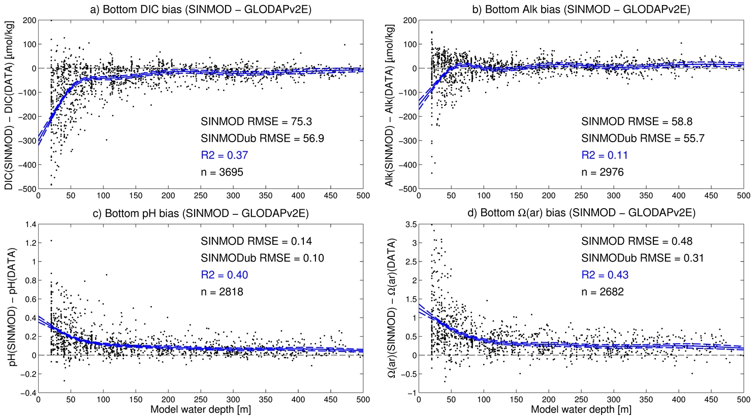
Figure 3. SINMOD regional bottom water biases for dissolved inorganic carbon (a), total alkalinity (b), total scale pH (c), and aragonite saturation state (d). Black dots show model-data errors for all GLODAPv2-extended data within the SINMOD pan-Arctic domain and within the test period 1984–2008. Blue lines show fitted spline bias functions (dashed lines are 95% CIs). Statistics in plots show the reduction in RMSE achieved by the bias-corrected model (“SINMODub”) as well as the R-squared values (R2) and sample sizes (n) for the bias function fits.
|
|
|